Continuous Probabilistic Cellular Automata
The code for this project can be found on its github repo
Introduction
I have to admit I find cellular automaton (CA) endlessly fascinating. They have never seemed to have found that killer real-world applications or ultimate deep insight; but I find the questions they raise about emergent behaviour and self organization incredibly engaging, that always keep me coming back to try out some new approach to exploring them.
In this post I’ll be looking at an extension to CA to allow for cells to be in a mixed state and probabilistic update rules to be applied.
1D Cellular Automata (Briefly)
To keep this post brief I’ll not go into too much depth of the theory on CA, if you’ve not encountered them before there’s a ton of stuff out there and as always wikipedia is a good place to start.
This project focused on 1-dimensional CA. This model can be imagined as a 1d array of cells, with each cell in a (usually discrete) state $s\in S$. At each update of the model, a cells state is updated based on its own state and local neighbourhood of cells. For example if each cell only considers it’s nearest neighbours then an update rule of a CA is the mapping
\[(s_{i-1}^{t}, s_{i}^{t}, s_{i+1}^{t}) \rightarrow s_{i}^{t+1}\]where $i$ indexes the cells position in the array and $t$ the step. The array is usually wrapped to form a closed loop (i.e. the end-cells are neighbours), and the evolution of the model visualized as a 2d space-time array where each row is one step of the model.

CA can have multiple states, and rules can be defined for various neighbourhoods around a cell, but in this case we will concentrate on 2-state and size 3 neighbourhood rules.
In many cases it’s convenient to index rules using the Wolfram system where the index is derived from the mapping represented in base $\vert S\vert$. For example if $S=\{0,1\}$ then full specifying the update rule requires a mapping for the $\vert S\vert^{3}=2^3$ possible triple states resulting in $2^8=256$ possible rules (See here for more details).
For example rule 110 is defined by the mapping
| $(s_{i-1}^{t}, s_{i}^{t}, s_{i+1}^{t})$ | 000 | 001 | 010 | 011 | 100 | 101 | 110 | 111 |
|---|---|---|---|---|---|---|---|---|
| $s_{i}^{t}$ | 0 | 1 | 1 | 1 | 0 | 1 | 1 | 0 |
A CA is then parameterized by an update rule, an initial state (common choice are a single live cell, or a random initial state) and topology of the array (i.e. a closed loop of fixed boundary conditions).
Motivation
This project was motivated by a couple of broad questions that have motivated a great deal of research on 1d CA:
-
Is there some way to classify the long term behaviour of CA? If one looks at all the possible rules configurations (for a chosen CA configuration) the dynamics of rules seem to roughly fall into 4 categories
- Evolution to a static homogeneous state
- Periodic behaviour where cells oscillate between states at each step or stable inhomogeneous structures
- Evolution to chaotic or seemingly noisy patterns
- Formation of localised persistent structures that can interact
though some rules can overlap some of these behaviors, and can obviously also depend on the initial state chosen. How can these classifications be made rigorous (or is there an underlying statistics or feature that classifies rules) and what forms the boundary between these behaviours?
Of particular interests are rules where stable structures form against a chaotic background, and such states can propagate and interact. For exmample it has been shown that rule 110 is turing complete.
-
In the case where structures do form, how do they form and persist against the background of chaotic noise? Is there some necessary condition for their formation and how do they propagate information and interact?
Note: These are a very brief outline of some of the interesting topics on the subject. There’s really a lot of interesting work covering these topic and more!!
Interesting work has been done on how changes in the initial state change the long term behaviour of the model (an analogue of the Lyapunov exponent used to study chaotic systems) and how information propagates through the array. It would seem expedient then to be able to express the initial state as a distribution across initial states or as something like a random walk that evolves over time as the update rule is applied to it.
This motivates being able to model a CA where the state of a cell can be a probability distribution on the state space (or maybe this could be thought of a superposition of states as in QM, though without any phase information). As the update rule is applied to a neighbourhood of cells, this also requires that we are able to model the joint or conditional probability of neighbouring cells.
Theory
Note: In the literature “Probabilistic CA” seems to refer to a model where the update rule is probabilistic but each cell still always has a fixed discrete state. So for now the name “Continuous Probabilistic CA” seems like a good name to distinguish from this
Probabilistic States
We’ll consider a model where each cell has a probability of being in a state $s$ denoted as
\[P(s_{i}^{t})=P(s_{i}^{t}=s)\quad\text{where}\quad s\in S\]The update rule applies to a cell, and its left and right neighbours. The probability of the cell being in a state at the next step is then given by
\[P\left(s_{i}^{t+1}\right)=\sum_{f=s_{i}^{t+1}}P\left(s_{i-1}^{t},s_{i}^{t},s_{i+1}^{t}\right)\]where the r.h.s is the joint probability of a state of the preceding triple and the summation is performed over the triples will result in the state $s_{i}^{t+1}$, i.e. when
\[f\left(s_{i-1}^{t},s_{i}^{t},s_{i+1}^{t}\right)=s_{i}^{t+1}\]for all combinations of the preceding states and $f(\dots)$ is the CA update function.
Note: The joint probability is important here as for certain rules neighbouring cells cannot be in certain configurations and as such should not be treated independently
This approach is ok for one step of the model but to repeatedly perform this update for an arbitrary number of steps we need the joint probability of two neighbouring cells at each site, and its neighbour to the right for each time step
\[P\left(s_{i}^{t}, s_{i+1}^{t}\right)\]extending the above approach for the update of a single cell gives
\[P\left(s_{i}^{t+1}, s_{i+1}^{t+1}\right)=\sum_{f=s_{i}^{t+1}, f=s_{i+1}^{t+1}}P\left(s_{i-1}^{t},s_{i}^{t},s_{i+1}^{t},s_{i+2}^{t}\right)\]the summation now over the overlapping triple cell states that will create the joint state. Then using the chain rule of probabilities we can decompose this to
\[\begin{align} P\left(s_{i}^{t+1}, s_{i+1}^{t+1}\right) &=\sum_{f} P\left(s_{i}^{t},s_{i+1}^{t}\right)P\left(s_{i-1}^{t}\vert s_{i}^{t}\right)P\left(s_{i+2}^{t}\vert s_{i+1}^{t}\right)\\ &=\sum_{f} P\left(s_{i-1}^{t},s_{i}^{t}\right)P\left(s_{i+1}^{t},s_{i+2}^{t}\right)h\left(s_{i}^{t},s_{i+1}^{t}\right) \end{align}\]where
\[h\left(s_{i}^{t},s_{i+1}^{t}\right)=\frac{P\left(s_{i}^{t},s_{i+1}^{t}\right)}{P\left(s_{i}^{t}\right)P\left(s_{i+1}^{t}\right)}\]This form is then useful as we need only store the joint probabilities for each cell (and it’s neighbour) and can obtain $h$ from this and the marginal probabilities.
Finally for the starting state at $t=0$ we assume that the initial probabilities are independent such that the initial array of joint probabilities can be found using
\[P\left(s_{i}^{0},s_{i+1}^{0}\right)=P\left(s_{i}^{0}\right)P\left(s_{i+1}^{0}\right)\]Probabilistic Update Rules
In the above model, any uncertainty in the model can only arise from uncertainty in the initial state (if all the cells are in only one state initially i.e. $P(s)\in\{0,1\}$ it behaves like a regular CA), as the update rule still maps discrete states to discrete states.
We can extend the model to include probabilistic updates, represented by the conditional distribution
\[P\left(s_{i}^{t+1}, s_{i+1}^{t+1}\:\vert\: q_{i}^{t}\right)\]where $q_{i}^{t}$ is the preceding quadruple of states that inform the updated joint probability
\[q_{i}^{t} = \left(s_{i-1}^{t},s_{i}^{t},s_{i+1}^{t},s_{i+2}^{t}\right)\]this actually somewhat simplifies the form of the summation to give
\[\begin{align} P\left(s_{i}^{t+1}, s_{i+1}^{t+1}\right) &= \sum_{q_{i}^{t}}P\left(s_{i}^{t+1}, s_{i+1}^{t+1}\:|\:q_{i}^{t}\right)P\left(q_{i}^{t}\right)\\ &= \sum_{q_{i}^{t}}P\left(s_{i}^{t+1}, s_{i+1}^{t+1}\:|\:q_{i}^{t}\right)P\left(s_{i-1}^{t},s_{i}^{t}\right)P\left(s_{i+1}^{t},s_{i+2}^{t}\right)h\left(s_{i}^{t},s_{i+1}^{t}\right) \end{align}\]where the summation is over all the possible patterns of the preceding quadruples cells.
In the case that
\[P\left(s_{i}^{t+1}, s_{i+1}^{t+1}\:\mid \: q_{i}^{t}\right) \in \{0,1\}\]then a deterministic CA rule is recovered.
Implementation
This was straightforward enough to implement in numpy. As with most cellular automata models like this (where the update is done in parallel for all cells) the real trick is shifting the state array left and right to be able to vectorize the update step.
The model is specified by 3 parameters (as in a regular CA):
-
The initial state of the cells, in this case it has the dimensions $\text{steps}\times\vert S\vert$ specifying the initial probability distribution for each cell
-
The update rule, provided as a 2d array mapping the permutation of triples to the probability of the update state. This represents:
\[P\left(s_{i}^{t+1}\:\vert\: s_{i-1}^{t}, s_{i}^{t}, s_{i+1}^{t}\right)\] -
The number of steps to run the model for
In brief the models then follows the following steps:
-
Use the rule array to generate an array representing the update of joint probabilities conditioned on the preceding quadruples of cells
\[P\left(s_{i}^{t+1}, s_{i+1}^{t+1}\:\vert\: q_{i}^{t}\right)\] -
Initialize an empty array for joint probabilities with the shape
\[\text{steps}\times \text{width}\times \vert S \vert\times\vert S \vert\](i.e. a joint probability distribution for each cell and for each step of the model)
- Set the initial joint probability row from the initial state, using the independence of the initial states
- At each step calculate the marginal probabilities required to calculate $h\left(s_{i}^{t+1},s_{i+1}^{t+1}\right)$ along with the left and right shifted rows for $P\left(s_{i-1}^{t},s_{i}^{t}\right)$ and $P\left(s_{i+1}^{t},s_{i+2}^{t}\right)$
- For each joint probability entry sum over all the contributions from the combinations of the preceding quadruple of cells
Complexity and Numerical Underflow
Computationally there are a couple of potential drawbacks
- Computational complexity: Increasing the number of states increases both the storage space required and the complexity of the update calculation. The number of states means scaling the array of joint probabilities like $\vert S\vert^2$ for each cell. When then need to then perform the update for each of these new entities as well as including contributions for the additional permutation of states which scale as $\vert S\vert^4$.
- Numerical Underflow: As with many models where probabilities are
repeatedly multiplied numerical underflow can occur. A common approach is
to work with log probabilities and use techniques like the
log-sum-exp trick.
In this case there a couple of things that make this tricky:
- The lack of a well-defined 0 probability in log space prohibits using binary states as inputs to the model
- Calculating the marginal probabilities required in the update step still means moving between log and normal probabilities which does not aid in reducing numerical under/overflow
Analysis/Plotting
Plotting the result of the model as a time-space diagram like a regular CA requires aggregating the joint probability distribution of each cell in some manner, but I also looked to choose statistics that might reveal underlying dynamics of the probabilistic CA:
-
The probability distribution for each cell are easily recovered as the marginals of the joint distribution
\[P\left(s_{i}^{t}\right)=\sum_{s_{i+1}^{t}}P\left(s_{i}^{t}, s_{i+1}^{t}\right)\] -
The mutual information of the joint probabilities also seems like it should be a useful, giving something like mutual dependence between neighbouring cells. Here defined for a single cell as
\[I_{i}^{t} = \sum_{s_{i}^{t}, s_{i+1}^{t}}P\left(s_{i}^{t}, s_{i+1}^{t}\right) \text{log}\left(\frac{P\left(s_{i}^{t}, s_{i+1}^{t}\right)}{P\left(s_{i}^{t}\right)P\left(s_{i+1}^{t}\right)}\right)\]
An additional issue is that in many cases the relative difference (of these statistics) between cells decreases over time, meaning plots can fail to adequately show features contained in resulting arrays. Applying min-max scaling across rows of the array is one approach used to tackle this issue, though care should be taken in how this is interpreted, given that small relative differences could also be a result of numerical precision.
Results
Given the large number of potential parametrizations of the model (mixing probabilistic update rules, and initial states) I looked to focus on two simple cases:
-
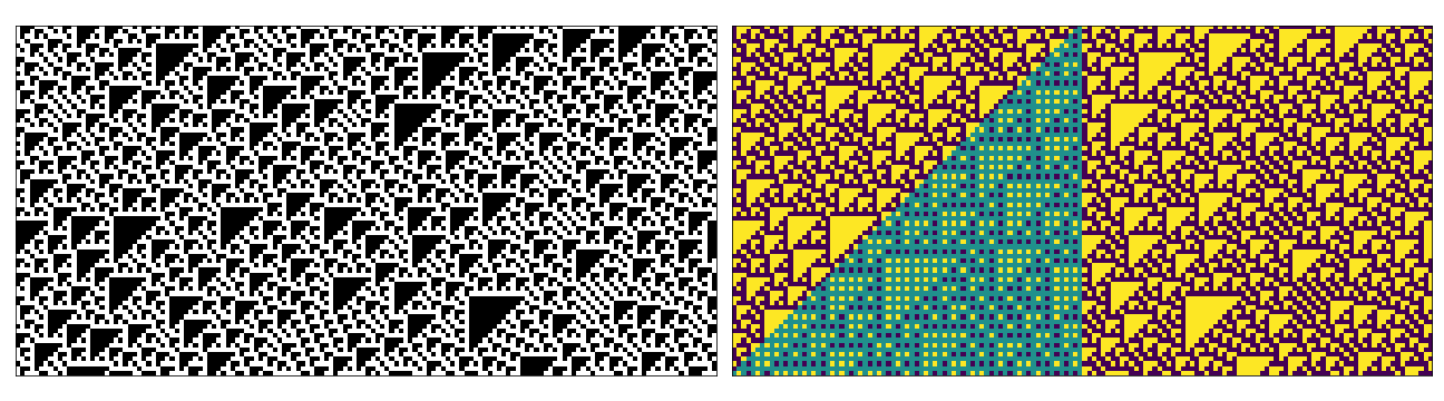
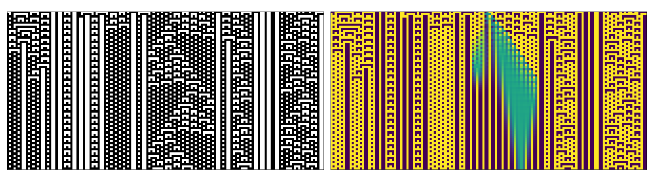
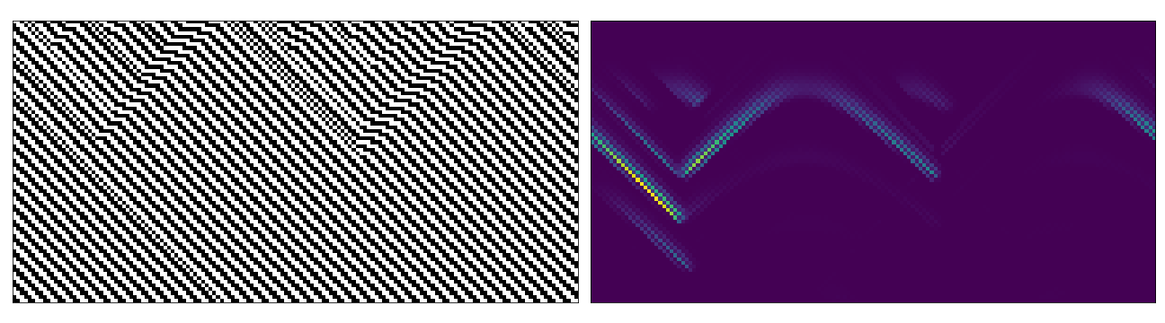
Standard update rules (i.e. deterministic) with a randomly chosen discrete initial state containing a single cell in a mixed state. Used to investigate how the uncertainty from a single cell propagates through the state over time.
-
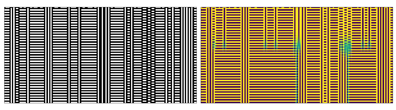
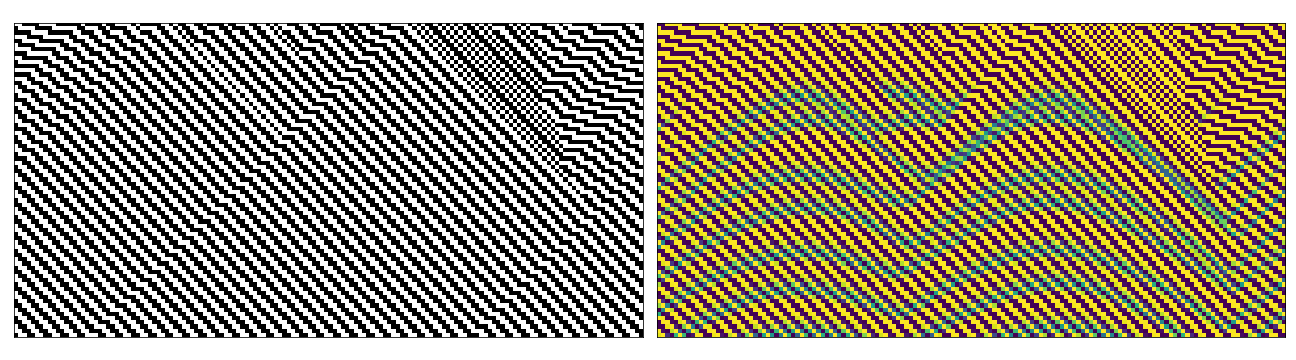
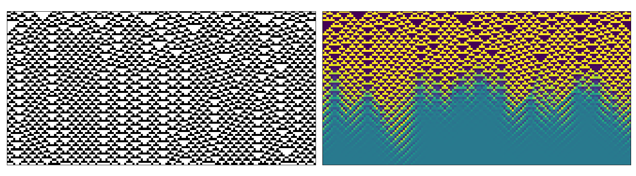
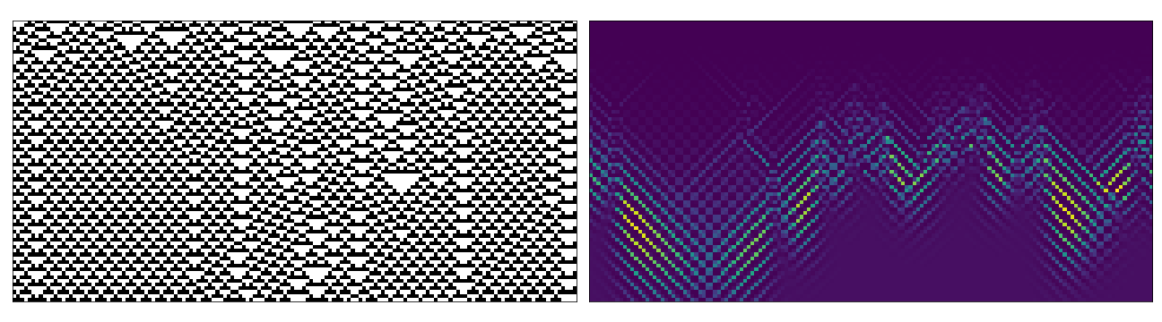
Update rules with the same perturbation applied to each mapping, and a randomly chosen discrete initial state. For example if the undeterred rule maps $(0,0,0) \rightarrow 0$ then the perturbed probabilities are $P(0\vert 0,0,0)=1-\epsilon$ and $P(1\vert 0,0,0)=\epsilon$ (applied to all the permutations). This could be thought of as a probability of error when applying the update rule, we can then consider how robust rules and patterns are to these errors.
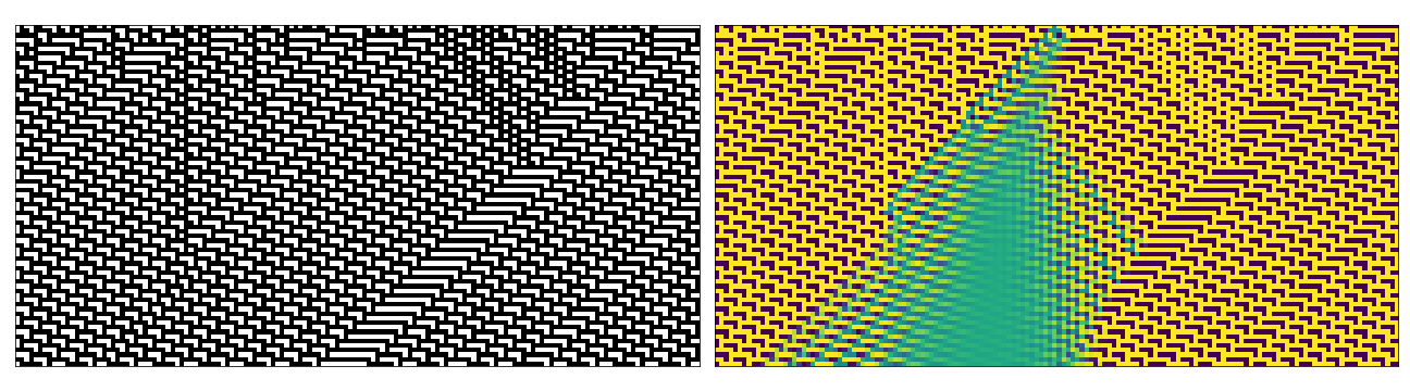
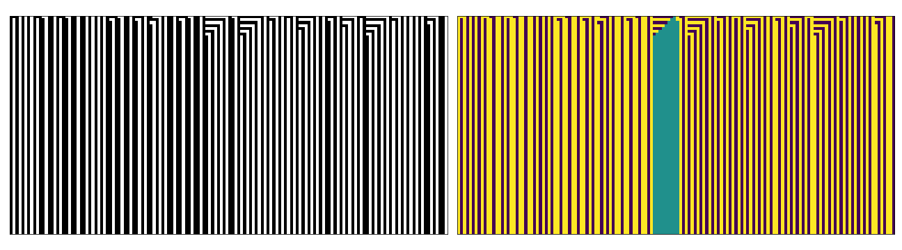
Below are some examples of space-time diagrams from these cases (though far exhaustive given the possible combinations of parameters). In each case the left image is the equivalent regular CA evolution (i.e. no perturbation in the update rule or initial state). The right hand side has been coloured to emphasise values between 0-1.
Perturbed Initial State
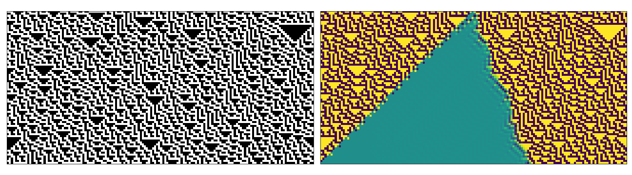
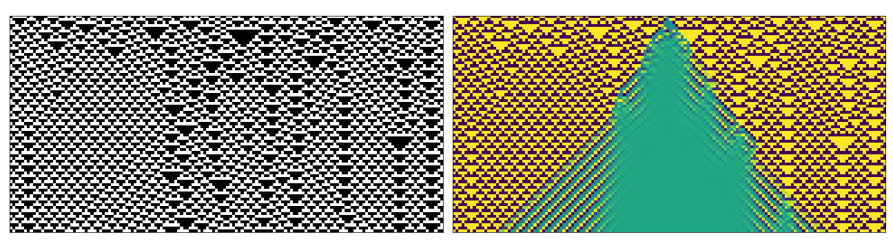
Perturbed Update Rule
Conclusion
In terms of a model, I feel this turned out quite well. Extending a regular CA into one that supports mixed/probabilistic cell states turned out to be quite a neat algorithm, and the resulting implementation relatively speedy. It’d be nice to have a robust way of working in log-probability space, but the current model seems relatively robust in most cases. Currently, the model-runner only supports binary states, but the extension to larger state spaces should be relatively straight forward.
Unfortunately the results are mostly qualitative, there seem to be some nice features revealed that point towards interesting dynamics and information propagation between cells. One could maybe make some statements about robustness of patterns, or the propagation of uncertainty relate to the classes of behaviours (described earlier in this post) but this is in need of further analysis.
One thing that might be nice to explore is the transition between the behaviour of update rules. Being able to apply probabilistic update rules means one could explore the continuous space of update rules inside the $\vert S\vert$-dimensional interval (of which the regular discrete CA rules form the corners).
At a minimum though, some of the images would make for cool album covers!
All the code needed to run the model and produce the plots included in this post is available here so please go ahead and try it out, it’d be interesting to see what other people come up with!