Cellular Automata Causal Regions
The code for this project can be found on it’s github repo
Introduction
This project was off-shoot of the work on probabilistic cellular automata the intention was to investigate how causal dependencies propagate through a 1d cellular automata (CA), and how these might inform identification of the behaviour of cellular automata.
Theory
If we consider cellular automata rules that only consider a cells nearest neighbours the ca update rule maps triples (of cells) to the state of the cell at the next step. We can represent the state of the cellular automata as triples, on graph that represents adjacent and overlapping triples, where an edge represent shifting a triple of cells to the left and appending the next state (the generalization of this concept is the de Bruijn Graph) i.e. if we move along the state array from left to right we are walking along the corresponding directed graph.
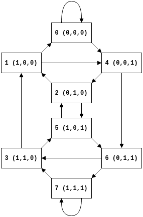
For different rules we can then look at how the rule maps triple to triples, for example rule 110 is defined by the mapping from triple to states:
| 000 | 001 | 010 | 011 | 100 | 101 | 110 | 111 |
|---|---|---|---|---|---|---|---|
| 0 | 1 | 1 | 1 | 0 | 1 | 1 | 0 |
then the possible updates for a triple-to-triples (as opposed to triples-to-states) from applying rule 110 can be represented by adjacency matrices:
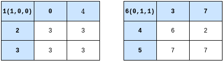
From this it should be clear that the state of a triple can be causally dependent on the previous state in 4 ways:
- The triple always maps to the same value, independent of the neighbourhood
- The next state of the triple depends on both it’s neighbours
- The next state of the triple depends on either it’s left or right neighbours only
We can then use this to examine the causal region that precedes a cell, that is if the state $s$ of triple at position $i$ at step $t$ of the model is $s_{i}^{t}$ then we say the causal region are preceding triples that the triple $s_{i}^{t}$ depends on. For example if the state of a triple $s_{i}^{t}$ is independent of its neighbours then it’s causal region contains $s_{i}^{t-1}$ (and we can then recursively follow this backward). If $s_{i}^{t}$ depends on only on it’s preceding left neighbour then the causal region contains $s_{i-1}^{t-1}$ and $s_{i}^{t-1}$.
Implementation
As usual this was quick to implement in numpy with some judicious use of slicing operations. The algorithm to generate plots showing the size of causal regions followed the following steps:
- Generated the phase space array for the basic CA model (i.e. the space-time state of cells).
- For each cell look-up it’s dependency on its neighbourhood. For each cell
assign it a pair containing it’s left and right dependency, where 0 indicates
the cell is only dependent on the previous cell and $\pm 1$ indicates the
cell is dependent on it’s neighbour.
For example:
( 0,0)indicates the cell only depends on the previous cell(-1,0)indicates the cell is dependent on the left (but not the right)( 0,1)indicates the cell is dependent on the right (but not the left)(-1,1)indicates the cell is dependent on the left and right
- Iterate forward over rows (i.e. time) and for each row, add the contributions from the previous row dependent on the causal dependence.
In the final step we are applying something like the following to each cell:
s[t][i][0] = s[t][i][0] + decay*s[t-1][s+s[t][i][0]][0]
s[t][i][1] = s[t][i][1] + decay*s[t-1][s+s[t][i][1]][1]
the decay term applies more weight to contributions from more recent rows,
and also means the size of the causal region does not just explode over time.
The result of this algorithm is a 3d array in the shape [steps][width][2]
where the final index is the size of the casual region in the left and right
directions on the array respectively. To be able to plot this means flattening
using some function that helps represent the underlying dynamics (this was also
a similar issue in the
probabilistic cellular automata
project). I attempted to try and capture both the magnitude of the causal
region and the imbalance between left and right causality and so settled
on
where $l_{i}^{t}$ and $r_{i}^{t}$ are the left and right dependencies respectively.
Results
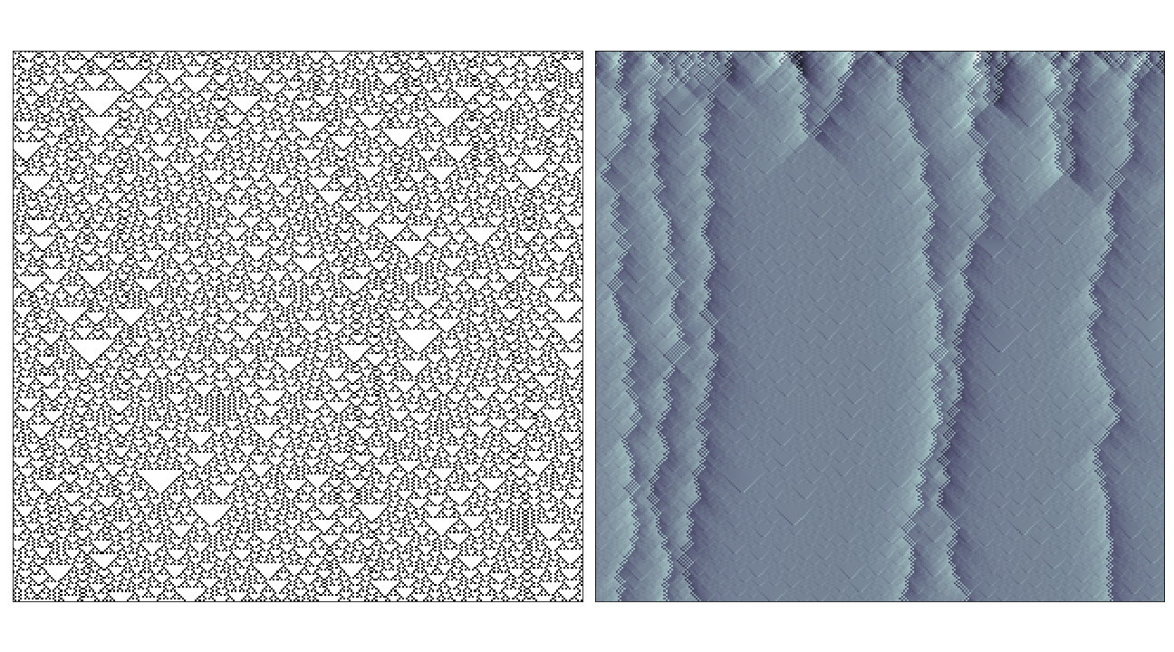
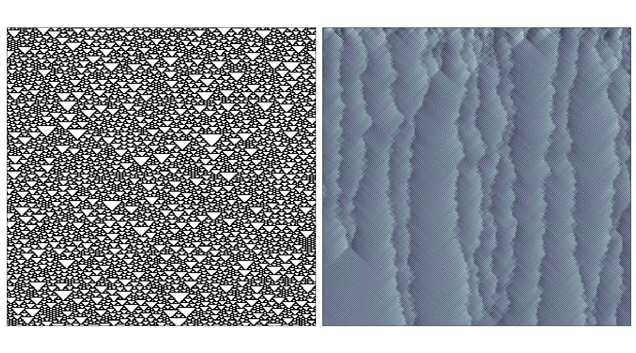
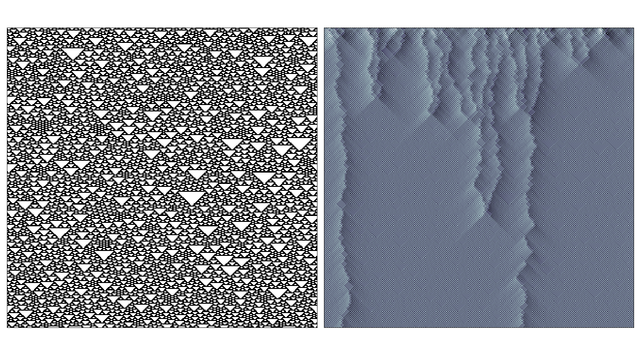
I’ve chery-picked some of the interesting examples here, in most cases where the rule has very simple behaviour (i.e. where the rule evolves to a fixed or oscillating pattern) the causal region plot doesn’t reveal much over the phase space-diagram. The most interesting cases seem to be where the rule generates propagating structures over complex/random regions, in these cases the causal regions seem to nicely pick out these structures from the background noise:
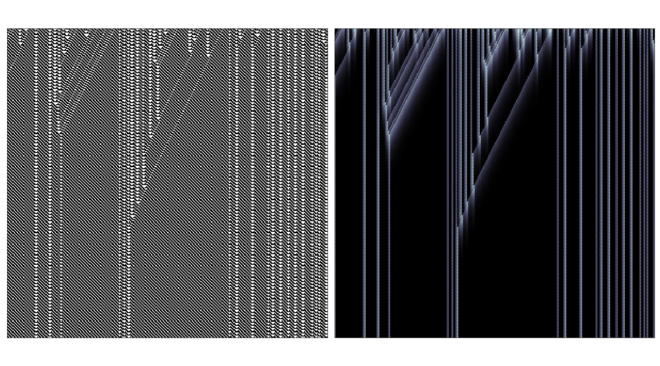
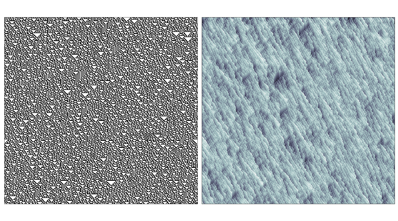
In the case of rules that produce totally chaotic behaviour, the causal region plot itself seems to contain the same amount of noise.
Conclusion
Like the probabilistic cellular automata project I feel the algorithm and implementation turned out really nicely but there was not a strong conclusion to be drawn from the results. As noted above in a few cases it seems to nicely pick out patterns from the background noise, but this is not general across the board.
I think part of this might be down to choice of function to flatten the causal information, this is one place where a better choice (or choice of plotting method might reveal more information) though it still seems like it would need to contain information on both the size of the preceding causal region and the dependence on direction.
As usual the code to produce these plots is available here with examples.