Continuous Probabilistic Cellular Automata Part 2: JAX and Differentiability
The code for this project can be found on its github repo
Introduction
This post extends previous work on probabilistic cellular automata (CA) that can be found in this post so have a read of that first.
TLDR: The dynamics of a CA are described by its update rule that maps the previous state of a cell, and its neighbours, to its updated state. In this extension cells are a probability distribution over possible states. The update rules then map probability distributions to probability distributions and the update rules themselves can be probabilistic.
Project Improvements
There have been two main updates:
Log Probability Distributions
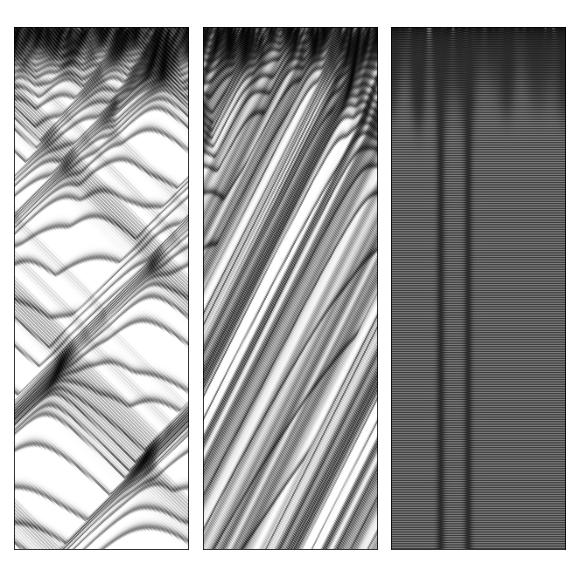
As noted in the previous post, due to the recursive nature of the CA, using state probabilities directly often results in numerical underflow as probabilities decay to small values. This can be avoided using log probabilities and techniques like the “log-sum-exp trick”.
The conversion to log probabilities turned out to be fairly straightforward, instead of the direct probabilistic update
\[\begin{align} P\left(s_{i}^{t+1}, s_{i+1}^{t+1}\right) = \sum_{q_{i}^{t}}P\left(s_{i}^{t+1}, s_{i+1}^{t+1}\:|\:q_{i}^{t}\right)P\left(q_{i}^{t}\right) \end{align}\]we can use
\[\begin{align} \text{log }P\left(s_{i}^{t+1}, s_{i+1}^{t+1}\right) &= \text{log }\sum_{q_{i}^{t}}P\left(s_{i}^{t+1}, s_{i+1}^{t+1}\:|\:q_{i}^{t}\right)P\left(q_{i}^{t}\right)\\ &= \text{log }\sum_{q_{i}^{t}}\text{exp}\left[\text{log }P\left(s_{i}^{t+1}, s_{i+1}^{t+1}\:|\:q_{i}^{t}\right) + \text{log}P\left(q_{i}^{t}\right)\right] \end{align}\]Once we expand $\text{log}P\left(q_{i}^{t}\right)$, we find we need to only store
\[\begin{align} \text{log }P\left(s_{i}^{t+1}, s_{i+1}^{t+1}\right) \end{align}\]as the state of the CA.
This allows for much better numerical stability (and larger executions as shown below), at the cost of not being able to represent absolute values like zero.
JAX Implementation
JAX is a Python high performance numerical computation library that has been around for a few years but seems to have recently gained a lot of popularity. There’s a lot to be said about it (I particularly really love the functional API) but it has two particularly killer features:
- Performance: JAX compiles to high performance code via XLA. The compilation and optimisation stage results in high performance CPU code, but can also compile to GPU or even TPU without changes to the code. In particular for this project this allows very fast execution of CA at large scales on GPU (speeding up the optimisation process detailed below).
- Gradients: Programs written using JAX can then (usually) be differentiated, and their gradients found (see here for more details). This has numerous applications across many areas of ML and mathematical modelling, but in this particular case we can look at differentiation of probabilistic cellular automata.
A notebook with examples of using this implementation can be found here.
Differentiability and Optimisation
The probabilistic CA effectively maps an update rule/distribution $R$ and initial distribution/state $S_{0}$ to an output series of states $S_{t}$:
\[\begin{align} C(R, S_{0}) \rightarrow S_{t} \end{align}\]Once implemented in JAX we can then calculate derivatives of the output with respect to inputs e.g.
\[\begin{equation} dS_{t}\mathbin{/}dR \quad\quad\text{or}\quad\quad dS_{t}\mathbin{/}dS_{0} \end{equation}\]In this example we will look at differentiating with respect to the update rule, and using this to optimise the rule using gradient descent.
For binary states the update rules is designated by 8 values, $R_{j}$, giving the probability of a previous state mapping to a new state
\[\begin{equation} R_{j} = P(S_{i}^{t+1}=1 | (S_{i-1}^{t}, S_{i}^{t}, S_{i+1}^{t})=j) \end{equation}\]where $j$ just maps the possible permutations of the previous states to integers.
We can then calculate $\partial S_{t}\mathbin{/}\partial R_{j}$, and use gradient descent to calculate iteratively update the rule
\[\begin{equation} R_{j}^{n+1} = R_{j}^{n} - \epsilon \frac{\partial L(S_{t})}{\partial R_{j}}(R^{n}, S_{0}) \end{equation}\]where $L(S_{t})$ here is some loss function on the output state.
Example
The code for this example can be found in this notebook.
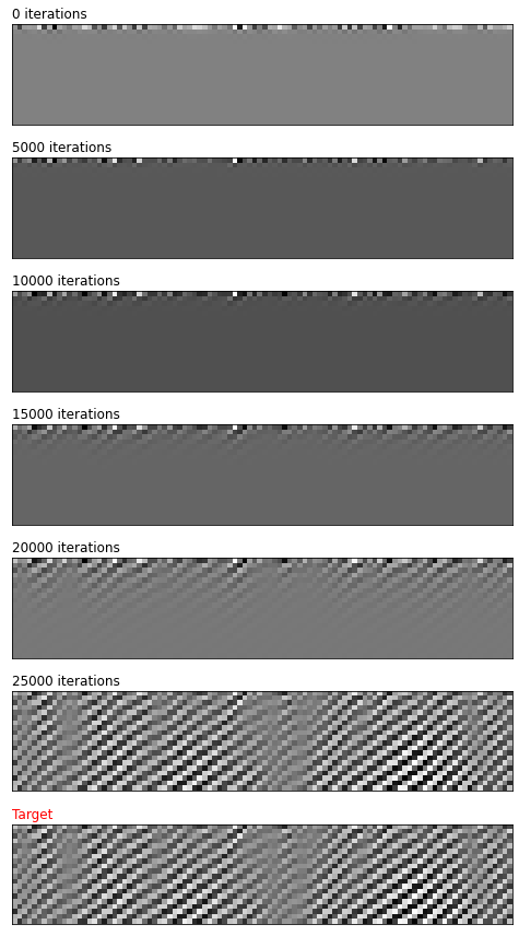
As a simple optimisation task we will generate a target outputs state, $S^{\prime}_{t}$ from a known ruleset and then starting from a random initial rule, move the rule towards the known rule using the loss function
\[\begin{equation} L(S_{t}) = \text{MSE}(S_{t}, S_{t}^{\prime}) \end{equation}\]The output generated by the CA over the course of training is shown below, along with the target distribution. We can see how the initial random state produces a mostly random output (as might be expected) but the target behaviour is revealed as we move towards the target ruleset.
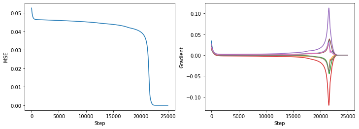
The change in loss, and gradients show some interesting behaviour (as shown below), training slows initially, before quickly converging after ~20,000 steps which is also reflected in the gradients of the individual rule components $R_{j}$
Conclusion & Next Steps
The combination of a proper log probability implementation and JAXs ability to differentiate (plus performance gain from JAX) turned out really nicely.
It’d now be nice to take this and see if optimisation can be used to find interesting probabilistic CA rules. From initial experimentation the hard part of this was designing a good loss function. The example here relies on having a known target, but what aggregate loss function will generate interesting CA rules? I suspect some interesting entropy measure, but need to do more work on what this might look like.
One are where this might be fruitful is for larger state spaces. The space of binary states is small enough to explore manually, but three states already becomes a much bigger space, being able to search this space effectively using gradient based methods may be an interesting result.